Data Importing, Tyding and Writing

R Training

Good Practice in Project Organization

When starting a new analysis, organize your work by creating a structured folder system:
📁 r_training
📂 scripts/ (code)
📂 data/ (datasets)
📁 outputs/ (results like plots, tables, etc.)

graph TD;
A[r_training] --> B[scripts];
A --> C[data];
A --> D[outputs];

graph TD;
A[r_training] --> B[scripts];
A --> C[data];
A --> D[outputs];

Note

Use lowercase and hyphens (-) instead of spaces when naming folders, files, and objects in R to maintain consistency and ease management.

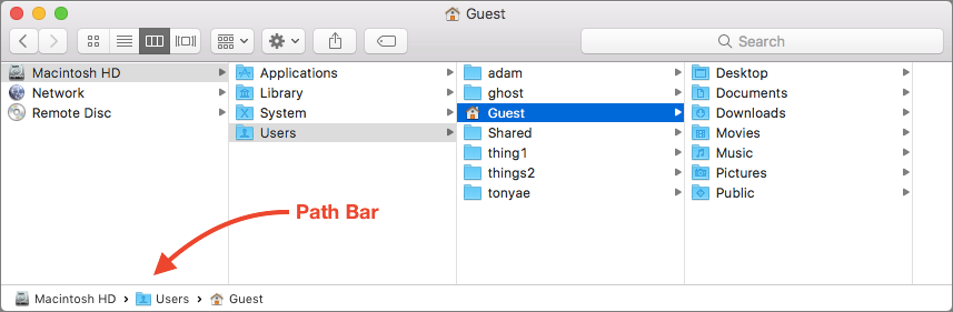
Understanding Folder Paths

A path is an address that tells a software where to find a file or folder on your computer.

Two Types of Paths:

Absolute Path: /Users/yourname/Desktop/r_training
Relative Path: r_training/scripts

The Advantage of Using Projects

R doesn’t automatically know where your files are. Using an RStudio project creates a shortcut that tells R where to find everything, making your workflow smoother.

Setting Up Your Environment

05:00

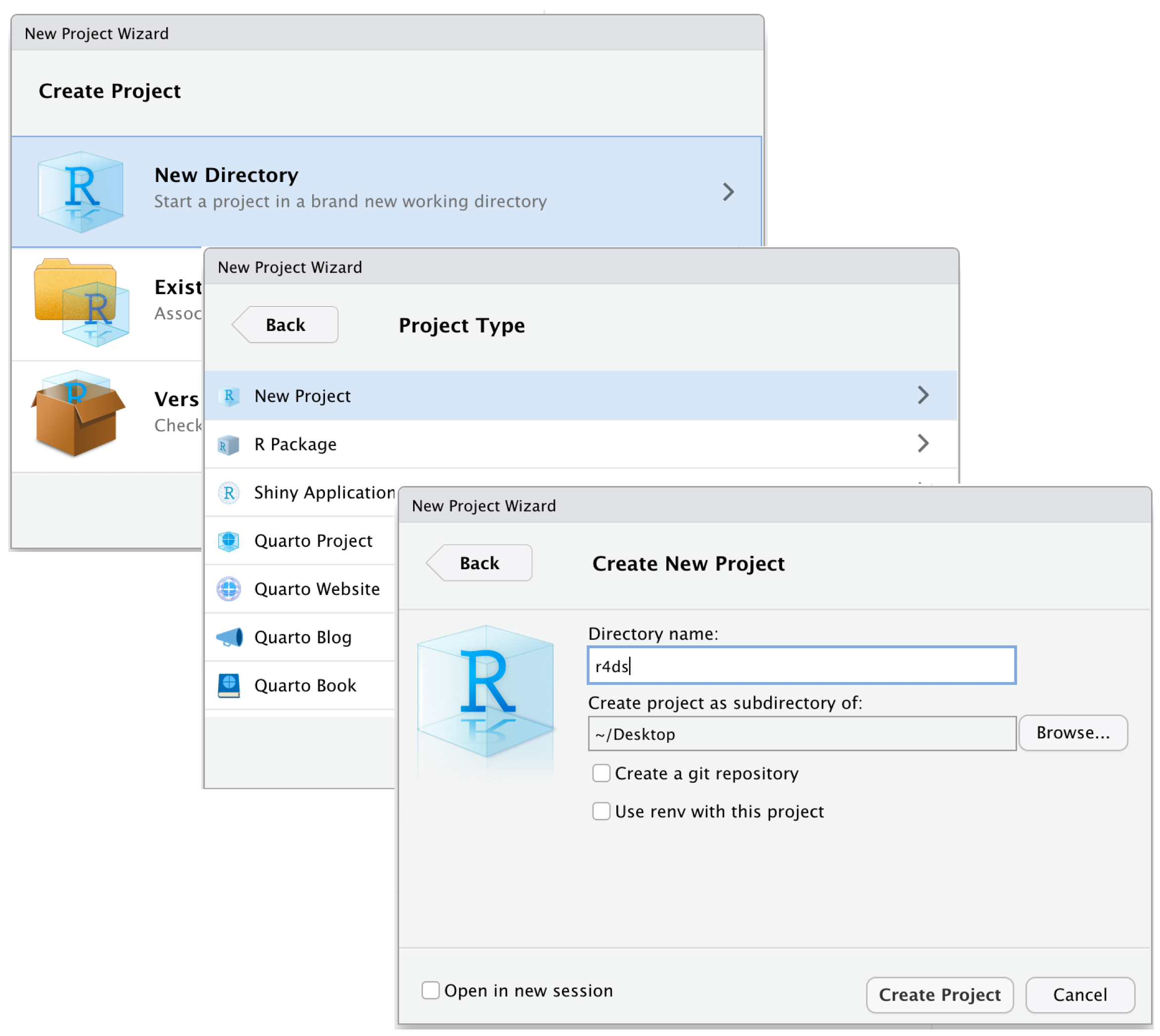
Create a new Folder named r_training
Create a Project

Open RStudio.
Go to File > New Project > Existing Directory.
Browse to your r_training folder and click Open.
Click Create Project to finish.

Open the Project (Double-click the file to open it in RStudio.)
Run this command in the RStudio Console:

usethis::use_course("https://github.com/your-organization/course-repo")

Follow the prompts to unzip the materials into your project folder.

You’re all set to begin! 🎉

Organizing the `data` Folder

graph TD;
A[data] --> B[Raw];
A --> C[Intermediate];
A --> D[Final];

graph TD;
A[data] --> B[Raw];
A --> C[Intermediate];
A --> D[Final];

`Raw`

Original, untouched data.
Backup recommended to preserve integrity.

`Intermediate`

Data formatted, renamed, and tidied.
Ready for further cleaning.

`Final`

Cleaned and transformed data.
Ready for graphs, tables, and regressions.

Import

Preparing Data for R: General Concepts and Best Practices

Document Types organizations extensively rely on spreadsheets (read)
Common data formats include:
Spreadsheets (.csv, .xlsx, xls…): Standard for structured data.
DTA (.dta): Used for data from STATA.
Spreadsheets
CSV is generally preferable:
Easier to import and process.
More compatible across different systems and software and much lighter.

Advanced

The Apache Arrow format is designed to handle large data sets efficiently, making it suitable for big data analysis. Arrow files offer faster read/write operations compared to traditional formats.

Importing Data into R

Main Import Methods
The library readxl provides some useful functions
read_xls() for XLS files (.xls).
read_xlsx() for Excel files (.xlsx).
read_csv() CSV files (.csv).
read_dta() for .dta files, using the haven package.
readRDS() for .RDS files.

Example: Importing an .xlsx File
To import an Excel file, you’ll need to load the readxl package

# Install the package if necessary
install.packages("readxl")

# Load the readxl package
library(readxl)

# Importing data from an .xlsx file
data <- read_excel("data_tax.xlsx")

Exercise 1: Data Import

You can find the exercise in the folder “Exercises/exercise_01_template.R”

10:00

Your tasks:

Load packages using pacman
Import three datasets:

firm_characteristics.csv (use fread)
vat_declarations.dta (use read_dta)
cit_declarations.xlsx sheet 2 (use read_excel)

For each dataset:

Display first 5 rows
Check column names
Clean names with janitor::clean_names()

Bonus: Ensure firm ID columns have the same name across all datasets

Exercise 1: Solutions

# Load packages
packages <- c("readxl", "dplyr", "tidyverse", "data.table", "here", "haven", "janitor")
if (!require("pacman")) install.packages("pacman")
pacman::p_load(packages, character.only = TRUE, install = TRUE)

# Load firm characteristics
dt_firms <- fread(here("Data", "Raw", "firm_characteristics.csv"))
head(dt_firms, 5)
names(dt_firms)
dt_firms <- clean_names(dt_firms)

# Load VAT declarations
panel_vat <- read_dta(here("Data", "Raw", "vat_declarations.dta"))
head(panel_vat, 5)
names(panel_vat)

# Load CIT declarations
panel_cit <- read_excel(here("Data", "Raw", "cit_declarations.xlsx"), sheet = 2)
head(panel_cit, 5)
names(panel_cit)

# Bonus: Ensure consistent naming
panel_vat <- rename(panel_vat, firm_id = id_firm)  # if needed

Inspecting Data

Inspecting Your Data: First Look

Once data is imported, we first want to take a look at it 👀

# print the first 5 rows
head(data)

# A tibble: 6 × 7
  `Taxpayer ID` Name       `Tax Filing Year` `Taxable Income` `Tax Paid` Region
  <chr>         <chr>                  <dbl>            <dbl>      <dbl> <chr> 
1 TX001         John Doe                2020            89854       8985 North 
2 TX001         John Doe                2021            65289       6528 North 
3 TX001         John Doe                2022            87053       8705 North 
4 TX001         John Doe                2023            58685       5868 North 
5 TX002         Jane Smith              2020            97152       9715 South 
6 TX002         Jane Smith              2021            62035       6203 South 
# ℹ 1 more variable: `Payment Date` <dttm>

# print the last 5 rows
tail(data)

# A tibble: 6 × 7
  `Taxpayer ID` Name        `Tax Filing Year` `Taxable Income` `Tax Paid` Region
  <chr>         <chr>                   <dbl>            <dbl>      <dbl> <chr> 
1 TX009         Olivia King              2022            91276       9127 North 
2 TX009         Olivia King              2023            90487       9048 North 
3 TX010         Liam Scott               2020            50776       5077 South 
4 TX010         Liam Scott               2021            86257       8625 South 
5 TX010         Liam Scott               2022            52659       5265 South 
6 TX010         Liam Scott               2023            76665       7666 South 
# ℹ 1 more variable: `Payment Date` <dttm>

# open the entire dataset 
# View(data)

Note

You might also notice that the Taxpayer ID and Full Name columns are surrounded by back-ticks. This is because they contain spaces, which breaks R’s standard naming rules, making them non-syntactic names. To refer to these variables in R, you need to enclose them in back-ticks.

Inspecting Your Data: Dimensions

Check the dimensions of your data:

# How many rows and columns?
dim(data)

[1] 40  7

# Number of rows
nrow(data)

[1] 40

# Number of columns
ncol(data)

[1] 7

Inspecting Your Data: Structure

Get column names and examine the data structure:

# List all column names
names(data)

[1] "Taxpayer ID"     "Name"            "Tax Filing Year" "Taxable Income" 
[5] "Tax Paid"        "Region"          "Payment Date"

# Or use colnames()
colnames(data)

[1] "Taxpayer ID"     "Name"            "Tax Filing Year" "Taxable Income" 
[5] "Tax Paid"        "Region"          "Payment Date"

# Check the structure in detail
str(data)

tibble [40 × 7] (S3: tbl_df/tbl/data.frame)
 $ Taxpayer ID    : chr [1:40] "TX001" "TX001" "TX001" "TX001" ...
 $ Name           : chr [1:40] "John Doe" "John Doe" "John Doe" "John Doe" ...
 $ Tax Filing Year: num [1:40] 2020 2021 2022 2023 2020 ...
 $ Taxable Income : num [1:40] 89854 65289 87053 58685 97152 ...
 $ Tax Paid       : num [1:40] 8985 6528 8705 5868 9715 ...
 $ Region         : chr [1:40] "North" "North" "North" "North" ...
 $ Payment Date   : POSIXct[1:40], format: "2020-01-31" "2021-12-31" ...

Inspecting Your Data: Better Structure View

Let’s get a better snapshot of the data structure and content:

# Install the package if necessary
# install.packages("dplyr")

# Load the dplyr package
library(dplyr)

# Get an overview of the data
glimpse(data)

Rows: 40
Columns: 7
$ `Taxpayer ID`     <chr> "TX001", "TX001", "TX001", "TX001", "TX002", "TX002"…
$ Name              <chr> "John Doe", "John Doe", "John Doe", "John Doe", "Jan…
$ `Tax Filing Year` <dbl> 2020, 2021, 2022, 2023, 2020, 2021, 2022, 2023, 2020…
$ `Taxable Income`  <dbl> 89854, 65289, 87053, 58685, 97152, 62035, 60378, 876…
$ `Tax Paid`        <dbl> 8985, 6528, 8705, 5868, 9715, 6203, 6037, 8768, 9368…
$ Region            <chr> "North", "North", "North", "North", "South", "South"…
$ `Payment Date`    <dttm> 2020-01-31, 2021-12-31, 2022-01-31, 2023-04-30, 202…

Tip

glimpse() is like str() but more readable! It shows data types, first few values, and fits nicely in your console.

Inspecting Your Data: Summary Statistics

Generate summary statistics for all columns:

# Get summary statistics
summary(data)

 Taxpayer ID            Name           Tax Filing Year Taxable Income 
 Length:40          Length:40          Min.   :2020    Min.   :50438  
 Class :character   Class :character   1st Qu.:2021    1st Qu.:58748  
 Mode  :character   Mode  :character   Median :2022    Median :78590  
                                       Mean   :2022    Mean   :75504  
                                       3rd Qu.:2022    3rd Qu.:90287  
                                       Max.   :2023    Max.   :98140  
    Tax Paid       Region           Payment Date                
 Min.   :5043   Length:40          Min.   :2020-01-31 00:00:00  
 1st Qu.:5874   Class :character   1st Qu.:2021-04-23 06:00:00  
 Median :7858   Mode  :character   Median :2022-01-15 12:00:00  
 Mean   :7550                      Mean   :2022-01-02 09:00:00  
 3rd Qu.:9028                      3rd Qu.:2023-01-07 18:00:00  
 Max.   :9814                      Max.   :2023-11-30 00:00:00

Tip

summary() is incredibly useful! For numeric variables, it shows min, max, mean, median, and quartiles. For character variables, it shows length and class.

Cleaning Column Names

Now, we’ll make sure that our variable names follow snake_case convention 😎

Option 1: Rename columns manually:

# We can rename columns one by one
data = rename(
  data, 
  tax_payer_id    = `Taxpayer ID`,
  name            = `Name`
  ...
)

Option 2: Automatically convert all column names to snake_case using janitor:

# Install the package if necessary
# install.packages("janitor")

# Load the janitor package
library(janitor)

# transform in snake_case all the var names
data = clean_names(data)

# take a look
names(data)

[1] "taxpayer_id"     "name"            "tax_filing_year" "taxable_income" 
[5] "tax_paid"        "region"          "payment_date"

Exercise 2: Inspecting Data

You can find the exercise in the folder “Exercises/exercise_02_template.R”

10:00

Your tasks:

Using the three datasets you imported in Exercise 1:

For dt_firms:

Check dimensions (rows and columns)
Use glimpse() to examine structure
Generate summary statistics

For panel_vat:

Display first 10 rows
Check number of unique firms
Find column names

For panel_cit:

Display last 5 rows
Check if there are any missing values using summary()

Exercise 2: Solutions

# Load required packages
library(dplyr)
library(data.table)

# 1. Inspect dt_firms
dim(dt_firms)
glimpse(dt_firms)
summary(dt_firms)

# 2. Inspect panel_vat
head(panel_vat, 10)
length(unique(panel_vat$firm_id))
names(panel_vat)

# 3. Inspect panel_cit
tail(panel_cit, 5)
summary(panel_cit)

Writing Data in R

Writing in .csv Format is (Almost) Always a Good Choice

For most cases, writing data in .csv format is a reliable and widely compatible option.
I recommend using the fwrite function from the data.table package for its speed and efficiency.

Below, we save various datasets into the Intermediate folder using fwrite:

# Write the VAT Data
fwrite(panel_vat, here("quarto_files", "Solutions", "Data", "Intermediate", "panel_vat.csv"))

# Write the CIT Declarations
fwrite(panel_cit, here("quarto_files", "Solutions", "Data", "Intermediate", "panel_cit.csv"))

# Write the Firm Characteristics
fwrite(dt_firms, here("quarto_files", "Solutions", "Data", "Intermediate", "dt_firms.csv"))

There other options to write data

Writing .rds Files (For R Objects)
The .rds format is specifically designed for saving R objects. It is useful for saving intermediate results, objects, or data.
We’ll explore this format in more detail later, but here’s a quick example:

# Example
base::saveRDS(data, "data_tax.rds")

Writing .xlsx Files (For Excel Compatibility): To save data in Excel format (.xlsx), use the writexl package. It is lightweight and doesn’t require external dependencies.

# Example
writexl::write_xlsx(data, "data_tax.xlsx")

Writing .parquet Files (For Large Datasets): The .parquet format is a columnar storage format that is highly efficient for both reading and writing large datasets (typically >1GB).

# Example
arrow::write_parquet(data, "data_tax.parquet")

# Reading parquet files
arrow::read_parquet("data_tax.parquet")

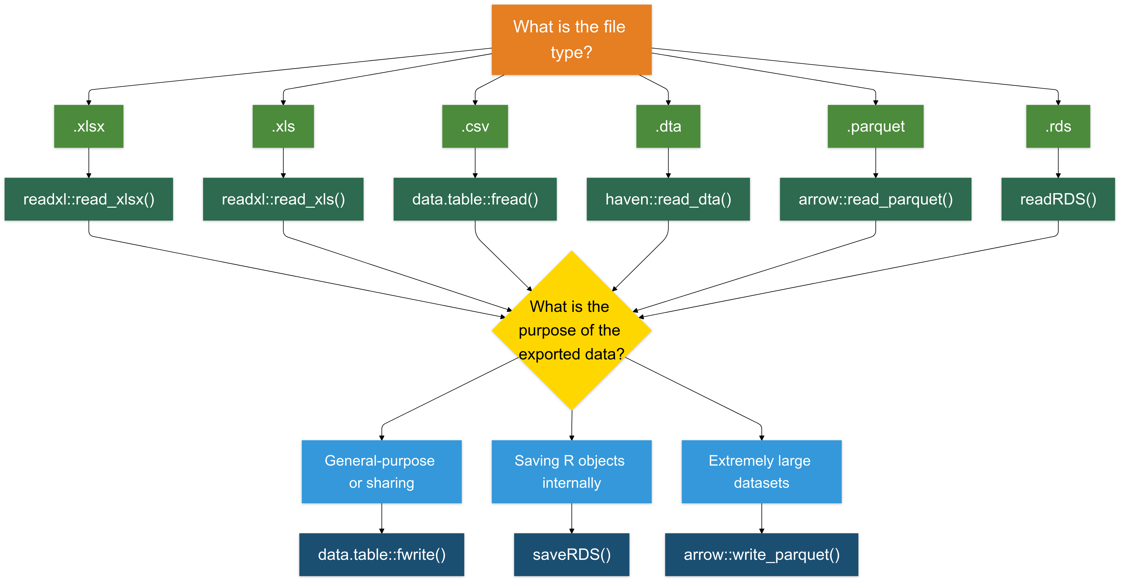
To Sum Up

Exercise 3: Write Clean Data

You can find the exercise in the folder “Exercises/exercise_03_template.R”

05:00

Your tasks:

Save the three cleaned datasets in different formats:

Firm characteristics → CSV
Save as data/intermediate/firms_clean.csv using fwrite()
VAT declarations → RDS
Save as data/intermediate/vat_clean.rds using saveRDS()
CIT declarations → Parquet
Save as data/intermediate/cit_clean.parquet using write_parquet()
Bonus: Why did we choose different formats for each dataset?

Exercise 3: Solutions

# Load required packages
library(data.table)
library(arrow)
library(here)

# Save firm characteristics as CSV
fwrite(dt_firms, here("data", "intermediate", "firms_clean.csv"))

# Save VAT declarations as RDS
saveRDS(panel_vat, here("data", "intermediate", "vat_clean.rds"))

# Save CIT declarations as Parquet
write_parquet(panel_cit, here("data", "intermediate", "cit_clean.parquet"))

# Bonus Answer:
# dt_firms (CSV): Reference data, human-readable, shared across departments
# panel_vat (RDS): Preserves R data types, faster loading in R workflows
# panel_cit (Parquet): Efficient columnar storage for large panel datasets

Bonus: Connecting `R` to Databases

Why Connect to Databases?
Data is often stored in centralized databases for enhanced security, accessibility, and management.
Traditional workflows might involve submitting data requests to IT teams, causing delays and limited flexibility for analysts.

The Power of R for Database Access
Using R, you can:
Query data directly and in real-time.
Import large datasets seamlessly into your R environment.

Warning

However, I suggest extracting the data using your SQL interface and then working with the extracted data in R.

Example: connecting to a database

# Load Packages
library(DBI) # this package is always needed
library(RMariaDB) # there are packages for each type of database (e.g. MySQL, PostgreSQL, etc.)

# Establish a connection to the database
con <- dbConnect(
  MariaDB(),
  host = "database.server.com",
  user = "your_username",
  password = "your_password",
  dbname = "tax_database"
)

# Query the database
tax_data <- dbGetQuery(con, "SELECT * FROM vat_declarations WHERE year = 2023")

# Disconnect when done
dbDisconnect(con)

Data Importing, Tyding and Writing

Good Practice in Project Organization

Understanding Folder Paths

The Advantage of Using Projects

Setting Up Your Environment

Organizing the data Folder

Raw

Intermediate

Final

Import

Preparing Data for R: General Concepts and Best Practices

Importing Data into R

Exercise 1: Data Import

Exercise 1: Solutions

Inspecting Data

Inspecting Your Data: First Look

Inspecting Your Data: Dimensions

Inspecting Your Data: Structure

Inspecting Your Data: Better Structure View

Inspecting Your Data: Summary Statistics

Cleaning Column Names

Exercise 2: Inspecting Data

Exercise 2: Solutions

Writing Data in R

Writing in .csv Format is (Almost) Always a Good Choice

There other options to write data

To Sum Up

Exercise 3: Write Clean Data

Exercise 3: Solutions

Bonus: Connecting R to Databases

Example: connecting to a database

Organizing the `data` Folder

`Raw`

`Intermediate`

`Final`

Bonus: Connecting `R` to Databases