Introduction to `R`: the basics

R Training

Welcome to the “Introduction to R Course”!

We will learn to use the R programming language!
Using administrative data familiar to tax administrations.

Some pre-requirements

❌ The training does not require any background in statistical programming.

✅ A computer with R and RStudio installed is required to complete the exercises.

✅ Internet connection is required to download training materials.

What is `R`?

R is a programming language with powerful statistical and graphic capabilities.

Why should we use `R`?

R is very flexible and powerful—adaptable to nearly any task, (data cleaning, data visualization, econometrics, spatial data analysis, machine learning, web scraping, etc.)

R is open source and free to use - allowing both you and your institution to save money!

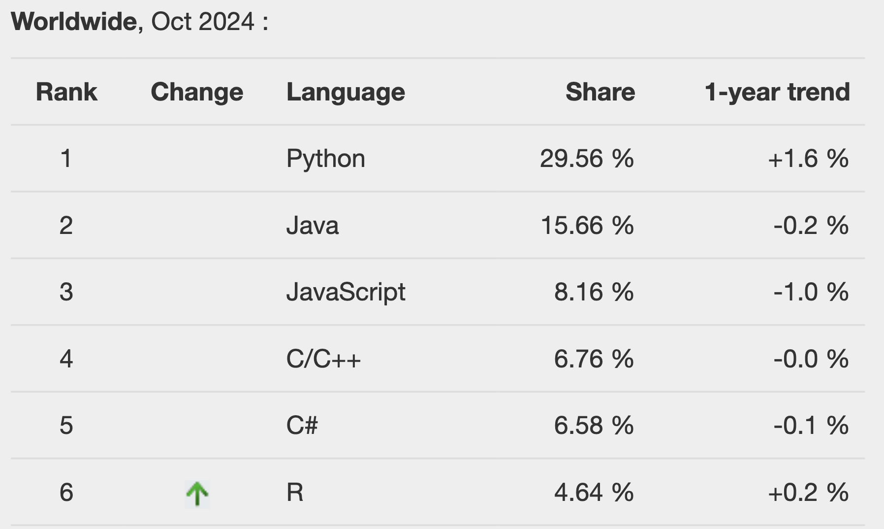
R has been growing rapidly in popularity.

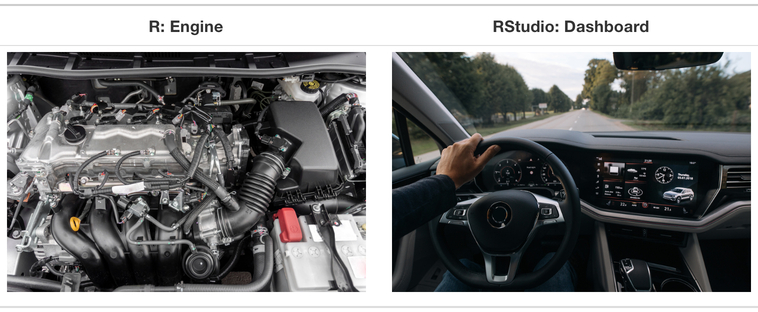
R offers a great interface - RStudio.

And what about `Excel`?

✅ Easy to use.

❌ Only good for small datasets.

❌ We don’t keep track of what we do.

❌ Not straightforward to merge data.

❌ And the list goes on…

And what about `STATA`?

✅ Stata is widely used in economics.

✅ Easy to learn.

❌ Only good for small datasets.

❌ Expensive!

❌ Lack of flexibility… do you hate keep, preserve, and restore too?

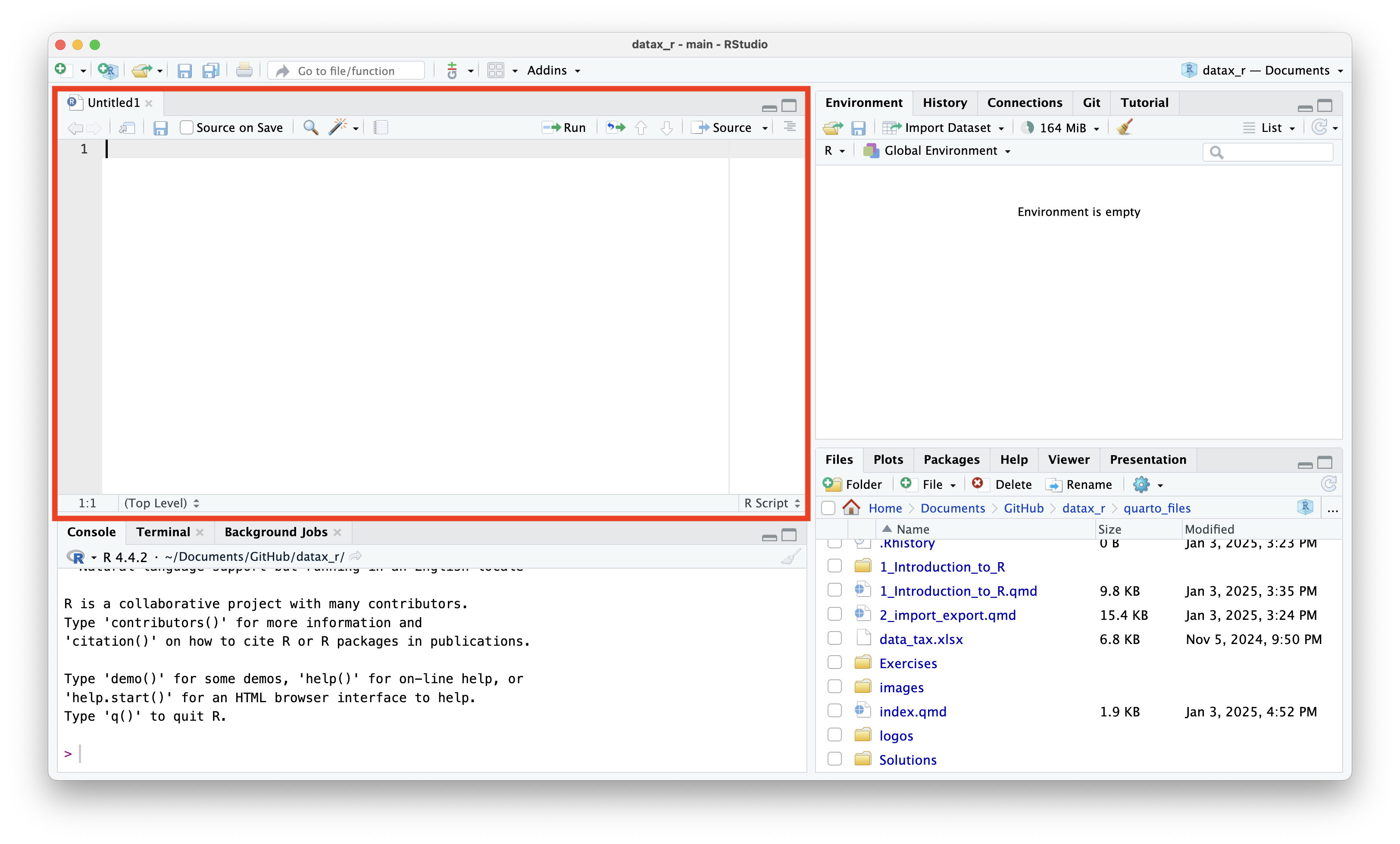
Getting Started with RStudio

You should see this!

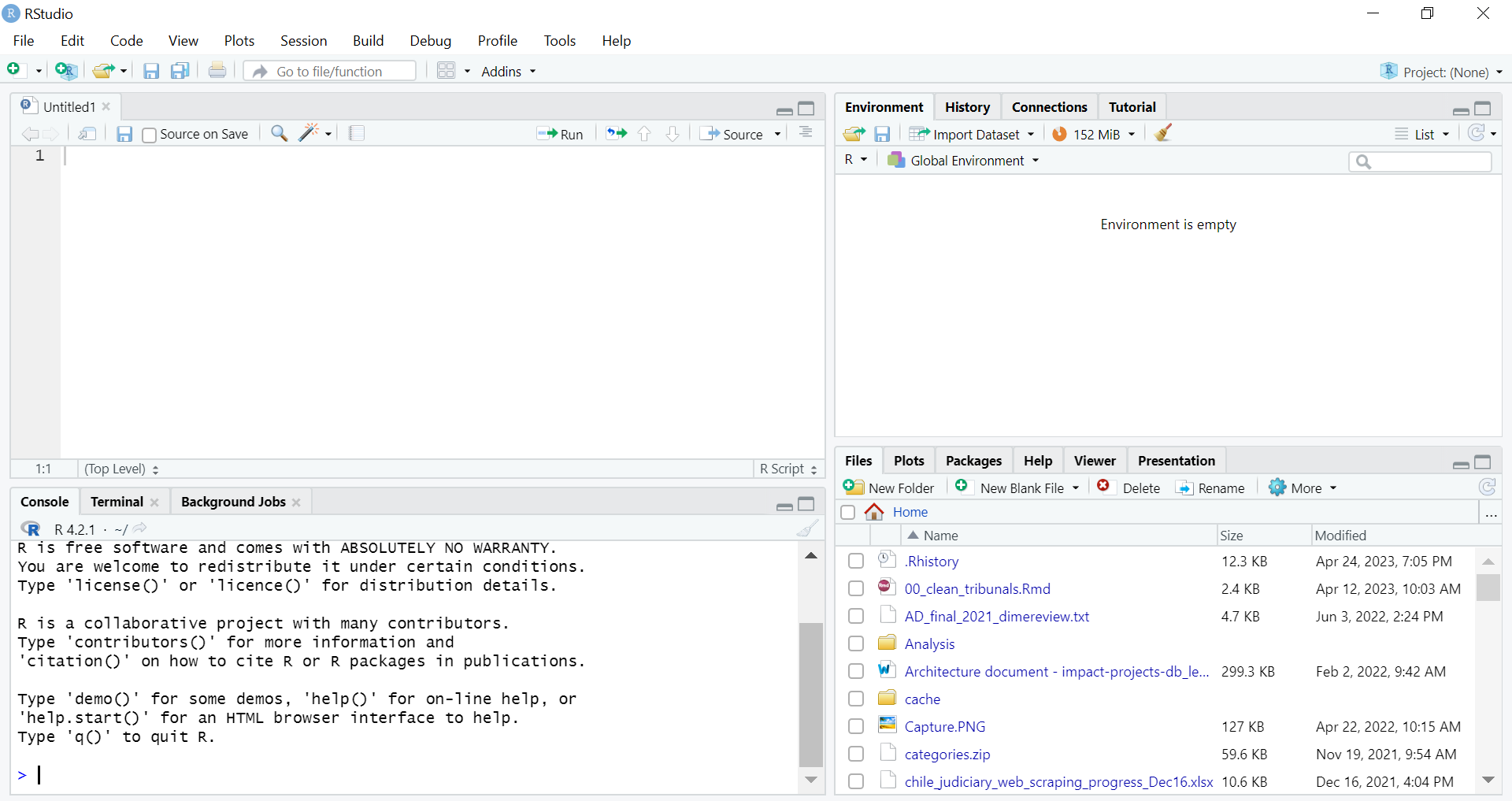
If you don’t, make sure you opened RStudio and not R!

Console

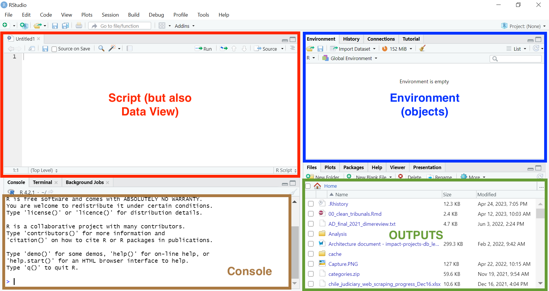
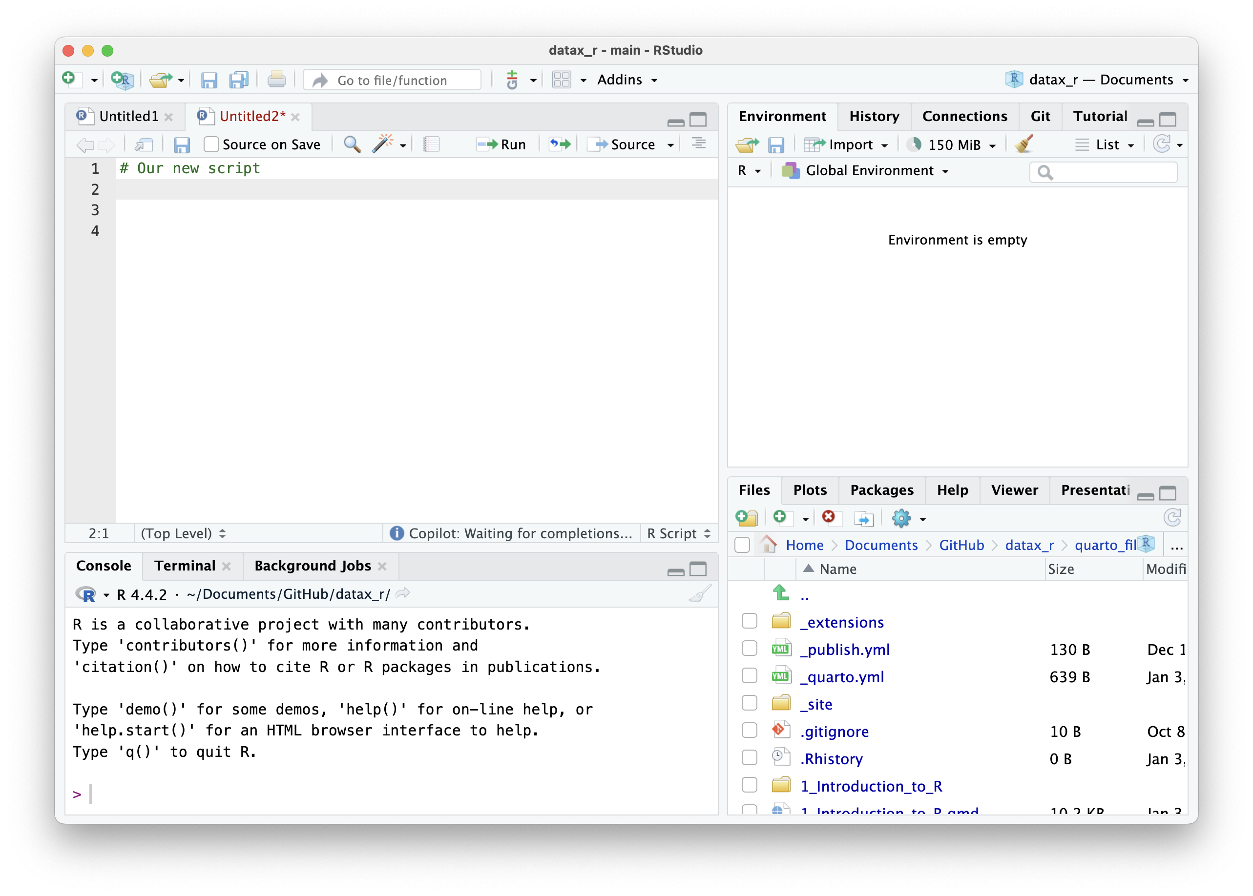
Let’s begin by writing your R scripts (source code) in the Source pane.

You can use the menubar or Ctrl + Shift + N to create new R scripts.

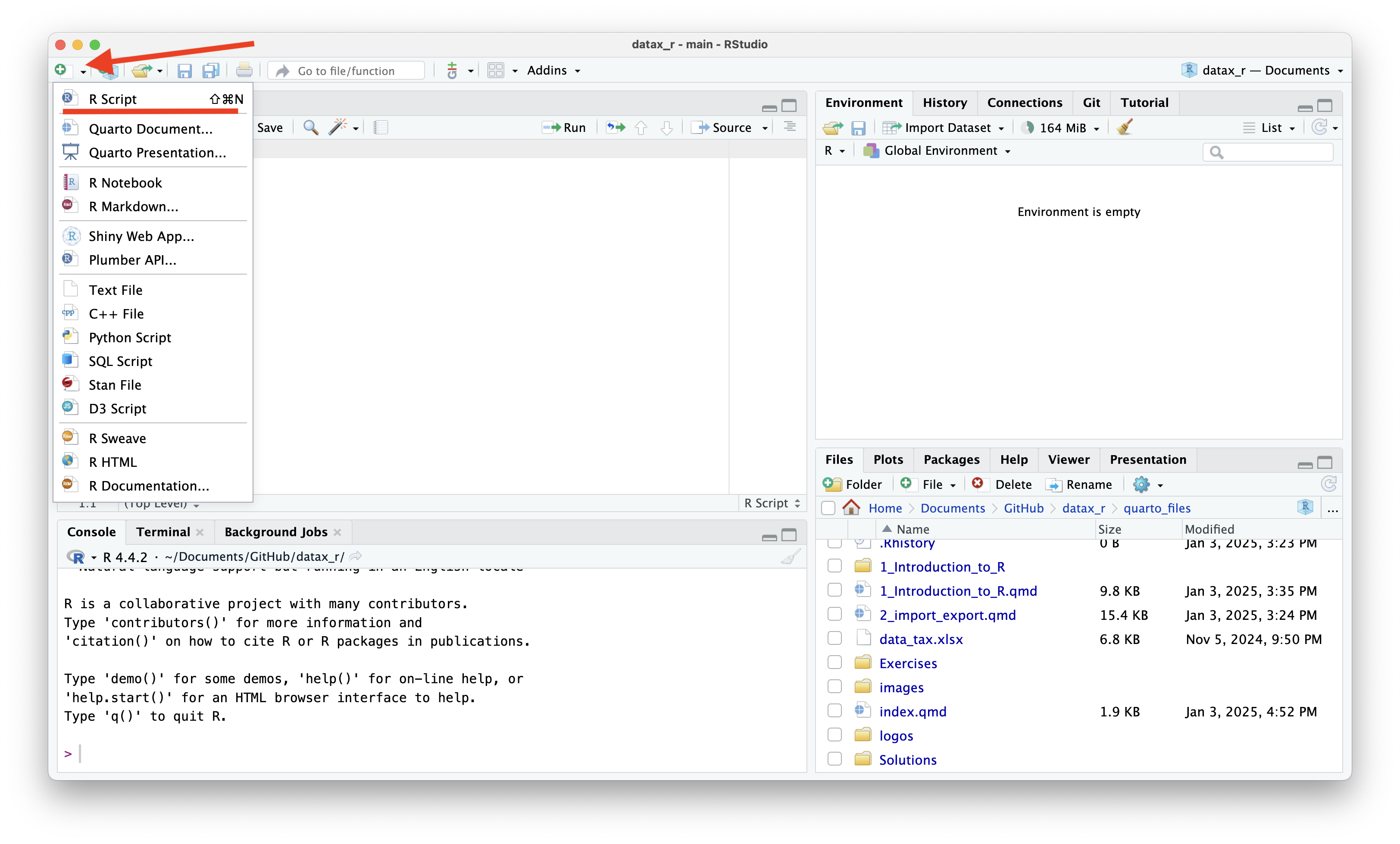
Scripts help us document and organize the steps we want to perform.

To run a command, type it in the Source pane and press Ctrl+Enter (Windows) to execute it in the Console.

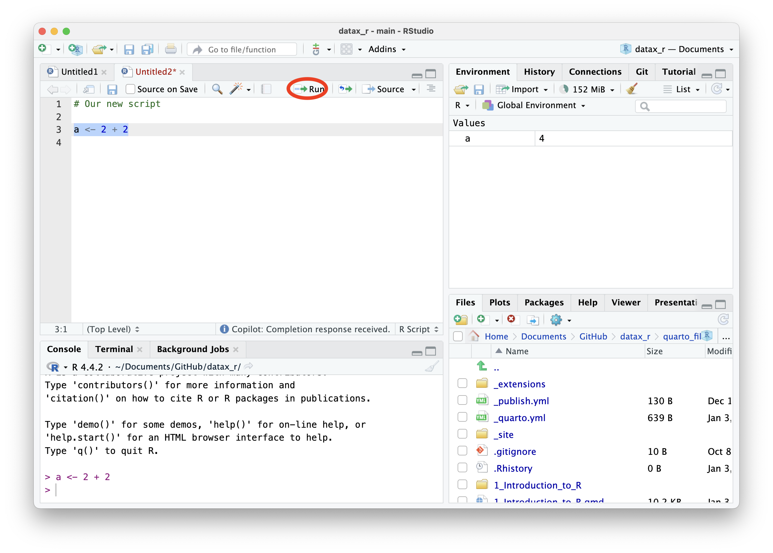
The result will appear in the Console pane (bottom-left panel).

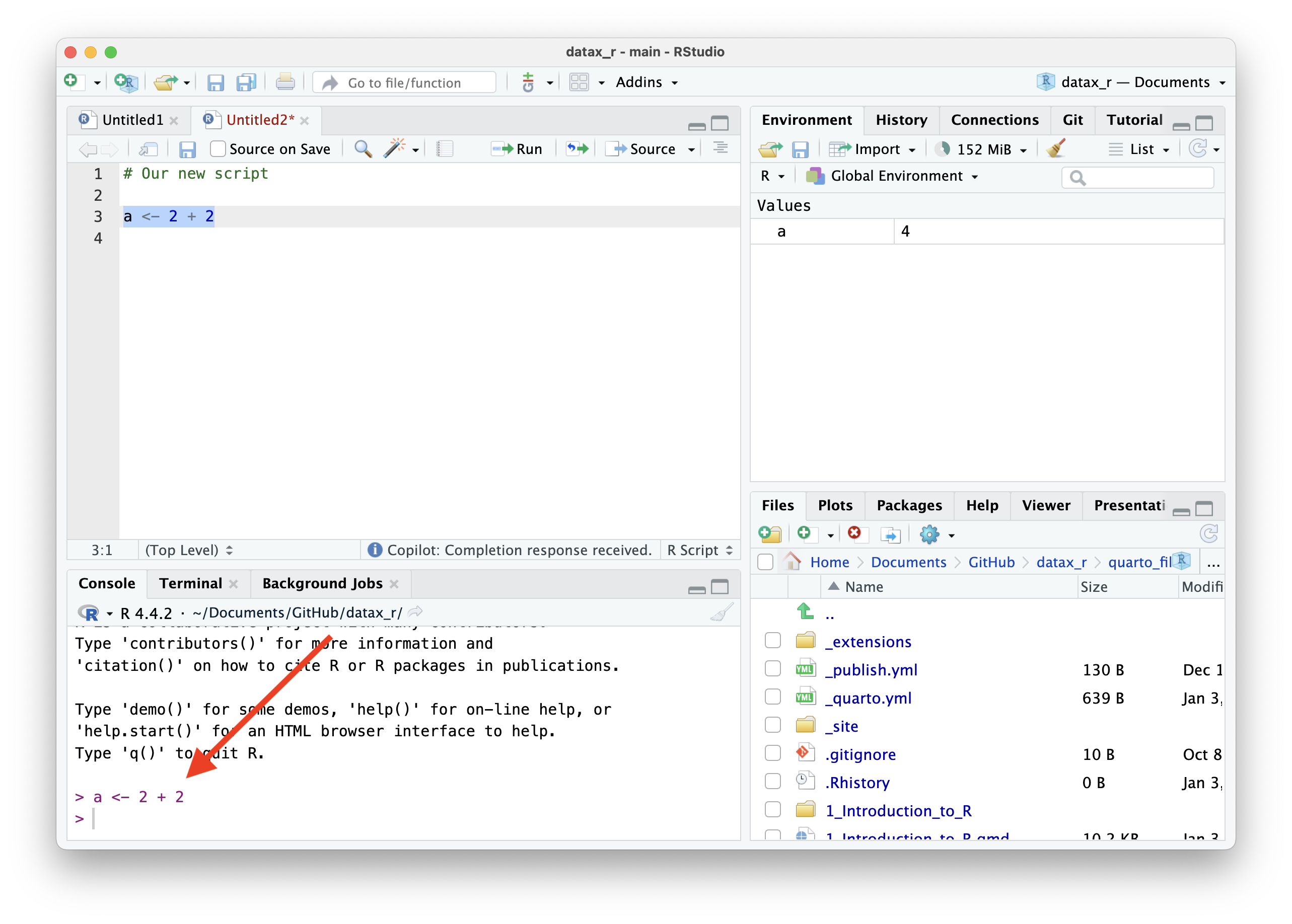
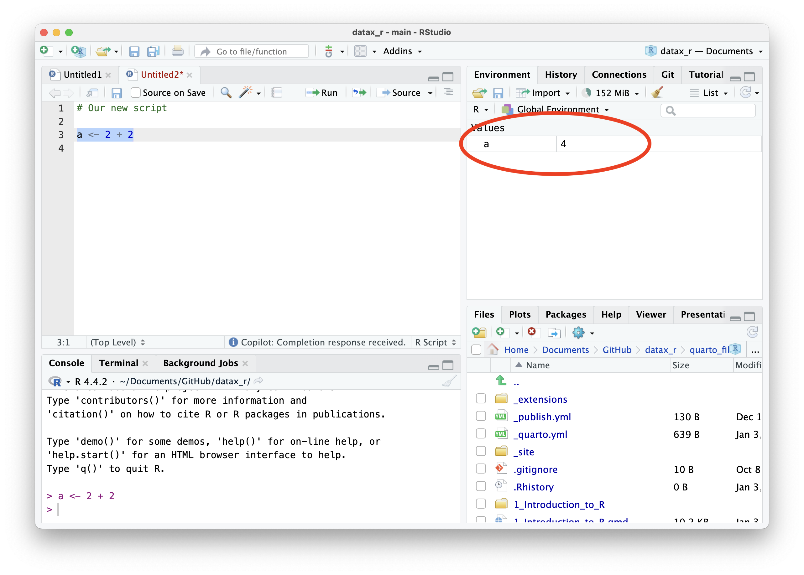
The Environment pane displays all the objects you’ve created during your session.

Using R as a Calculator

Basic Math Operations

A simple sum:

99 + 1

[1] 100

More complex calculations:

99 + 1 * 2

[1] 101

Following mathematical rules (order of operations):

(99 + 1) * 2

[1] 200

More Math Operations

Subtraction, multiplication, division:

150 - 50

[1] 100

10 * 5

[1] 50

100 / 4

[1] 25

Powers and square roots:

2^3       # 2 to the power of 3

[1] 8

sqrt(16)  # Square root

[1] 4

Scientific notation:

2 / 100000   # Very small number

[1] 2e-05

5e3          # 5000 in scientific notation

[1] 5000

Storing Results: Objects

Instead of just calculating, we can save results for later use.

vat_amount = 50000

Now we can use vat_amount in other calculations:

vat_amount * 1.10  # Add 10% penalty

[1] 55000

We can create multiple objects:

base_vat = 50000
penalty_rate = 0.10
total_vat = base_vat * (1 + penalty_rate)
total_vat

[1] 55000

Naming Rules for Objects

Use lowercase letters
Separate words with underscore (_) - this is called snake_case
Make names descriptive but not too long
Don’t use spaces or special characters

Good names:

vat_amount
firm_id
total_revenue_2024

Bad names:

VatAmount        # Mixed case
vat amount       # Has space (will cause error!)
x1               # Not descriptive
very_long_name_that_is_hard_to_type_and_read

Comments: Explaining Your Code

Use # to add comments - R will ignore everything after #

# This is a comment - R ignores this line

# Calculate VAT with penalty
base_vat = 50000        # VAT amount in local currency
penalty = base_vat * 0.05  # 5% penalty for late filing
total = base_vat + penalty
total

[1] 52500

Tip

Good practice: Comment your code to explain WHY you’re doing something, not just WHAT you’re doing.

Understanding Functions

What is a Function?

A function is a reusable piece of code that performs a specific task.

Think of functions as tools in a toolbox 🧰

Structure of a function call:

function_name(argument1, argument2, ...)

# sqrt() is a function that calculates square root
sqrt(16)

[1] 4

# round() is a function that rounds numbers
round(3.14159, digits = 2)

[1] 3.14

Function Arguments

Arguments are inputs to the function.

Positional arguments - order matters:

round(3.14159, 2)  # First = number to round, Second = decimal places

[1] 3.14

Named arguments - order doesn’t matter (recommended!):

round(x = 3.14159, digits = 2)

[1] 3.14

round(digits = 2, x = 3.14159)  # Same result!

[1] 3.14

Tip

Using named arguments makes your code clearer and less error-prone.

Common Mathematical Functions

# Absolute value
abs(-50)

[1] 50

# Logarithms
log(10)      # Natural log

[1] 2.302585

log10(100)   # Base 10 log

[1] 2

# Rounding
round(3.6)   # Round to nearest integer

[1] 4

ceiling(3.2) # Round up

[1] 4

floor(3.8)   # Round down

[1] 3

Getting Help with Functions

Three ways to learn about functions:

1. Help documentation:

help(round)   # Open help page
?round        # Shortcut

2. Examples:

example(round)  # See examples of how to use the function

3. Web search:

# Google: "R round function"
# Stack Overflow is your friend!

Important Functions You’ll Use Often

# Combining values
c(1, 2, 3, 4, 5)

# Creating sequences
seq(from = 1, to = 10, by = 2)

# Repeating values
rep(5, times = 3)

# Summary statistics (we'll use these soon!)
sum(...)
mean(...)
max(...)
min(...)

Data Types

Three Main Data Types

1. Numeric - numbers

vat_amount = 50000
penalty_rate = 0.05

2. Character - text (always in quotes)

firm_name = "ABC Corporation Ltd."
tax_id = "TIN-123456"

3. Logical - TRUE or FALSE

filed_on_time = TRUE
has_audit = FALSE

Checking Data Types

Use class() to check the type:

class(50000)

[1] "numeric"

class("Firm Name")

[1] "character"

class(TRUE)

[1] "logical"

Warning

Common mistake: Forgetting quotes around text

firm_name = ABC Corporation  # ERROR! R thinks ABC is an object
firm_name = "ABC Corporation"  # Correct!

Logical Operations (Comparisons)

Creating logical values through comparisons:

10 > 9    # Greater than

[1] TRUE

10 < 9    # Less than

[1] FALSE

10 == 9   # Equal to (note: two equal signs!)

[1] FALSE

10 != 9   # Not equal to

[1] TRUE

10 >= 9   # Greater than or equal to

[1] TRUE

10 <= 9   # Less than or equal to

[1] FALSE

Combining Logical Conditions

# AND: both conditions must be TRUE
10 > 9 & 9 < 10

[1] TRUE

# OR: at least one condition must be TRUE
10 > 9 | 9 > 10

[1] TRUE

# IN: check if value is in a set
9 %in% c(1, 5, 9, 10)

[1] TRUE

Tax example:

vat_amount = 75000

# Check if amount is in target range (50,000 to 100,000)
vat_amount >= 50000 & vat_amount <= 100000

[1] TRUE

Working with Vectors

What is a Vector?

A vector is a sequence of data elements of the same type.

Think of it like a column in a spreadsheet!

# Create a vector with c() function (combine)
vat_payments = c(45000, 67000, 89000, 52000, 91000)
vat_payments

[1] 45000 67000 89000 52000 91000

Note

All elements in a vector must be the same type (all numbers, all text, or all logical values).

Creating Different Types of Vectors

Numeric vectors:

vat_amounts = c(45500, 67200, 89100, 52800, 91300)
vat_amounts

[1] 45500 67200 89100 52800 91300

Character vectors:

firm_ids = c("FIRM_001", "FIRM_002", "FIRM_003", "FIRM_004", "FIRM_005")
firm_ids

[1] "FIRM_001" "FIRM_002" "FIRM_003" "FIRM_004" "FIRM_005"

Logical vectors:

filed_on_time = c(TRUE, TRUE, FALSE, TRUE, FALSE)
filed_on_time

[1]  TRUE  TRUE FALSE  TRUE FALSE

Useful Functions for Creating Vectors

Creating sequences with :

years = 2020:2024
years

[1] 2020 2021 2022 2023 2024

More control with seq()

# Every quarter from 1 to 12
quarters = seq(from = 1, to = 12, by = 3)
quarters

[1]  1  4  7 10

Repeating values with rep()

# Standard penalty rate for 5 firms
penalty_rate = rep(0.05, times = 5)
penalty_rate

[1] 0.05 0.05 0.05 0.05 0.05

How Many Elements? `length()`

firm_ids = c("FIRM_001", "FIRM_002", "FIRM_003", "FIRM_004", "FIRM_005")

# How many firms?
length(firm_ids)

[1] 5

Combining with sequences:

# Create IDs for 10 firms
all_ids = paste0("FIRM_", 1:10)
all_ids

 [1] "FIRM_1"  "FIRM_2"  "FIRM_3"  "FIRM_4"  "FIRM_5"  "FIRM_6"  "FIRM_7" 
 [8] "FIRM_8"  "FIRM_9"  "FIRM_10"

length(all_ids)

[1] 10

Vector Operations

Vector Arithmetic

R performs calculations element-by-element:

base_vat = c(50000, 75000, 90000, 45000, 82000)

# Add 10% penalty to all amounts
penalized_vat = base_vat * 1.10
penalized_vat

[1] 55000 82500 99000 49500 90200

Operations between two vectors:

declared = c(50000, 75000, 90000, 45000, 82000)
assessed = c(55000, 75000, 95000, 50000, 85000)

# Calculate differences
difference = assessed - declared
difference

[1] 5000    0 5000 5000 3000

Summary Statistics

Functions that work on entire vectors:

vat_collected = c(50000, 75000, 90000, 45000, 82000, 67000, 55000, 92000)

sum(vat_collected)      # Total

[1] 556000

mean(vat_collected)     # Average

[1] 69500

median(vat_collected)   # Middle value

[1] 71000

max(vat_collected)      # Highest

[1] 92000

min(vat_collected)      # Lowest

[1] 45000

Accessing Vector Elements: Indexing

Get a single element by position:

vat = c(50000, 75000, 90000, 45000, 82000)

# Get the 3rd element
vat[3]

[1] 90000

Get multiple elements:

# Get elements 2, 3, and 5
vat[c(2, 3, 5)]

[1] 75000 90000 82000

# Get first three elements
vat[1:3]

[1] 50000 75000 90000

Logical Indexing: Filtering Data

Find elements that meet a condition:

vat = c(50000, 75000, 90000, 45000, 82000)

# Which firms paid more than 60,000?
vat > 60000

[1] FALSE  TRUE  TRUE FALSE  TRUE

Use logical vectors to filter:

# Get only amounts above 60,000
high_vat = vat[vat > 60000]
high_vat

[1] 75000 90000 82000

Multiple conditions:

# VAT between 50,000 and 80,000
moderate_vat = vat[vat >= 50000 & vat <= 80000]
moderate_vat

[1] 50000 75000

Missing Values (NA)

Understanding Missing Data

In real tax administration data, missing values are common:

Firms that haven’t filed yet
Incomplete records
Data entry errors

In R, missing values are represented as NA (Not Available)

# Some firms haven't filed VAT declarations yet
vat_declared = c(50000, 75000, NA, 90000, 45000, NA, 82000)
vat_declared

[1] 50000 75000    NA 90000 45000    NA 82000

The Problem with NA

Math with NA returns NA!

# Try to calculate the mean
mean(vat_declared)

[1] NA

Warning

Any calculation involving NA will return NA unless you explicitly handle it!

Handling NA: The `na.rm` Argument

Most statistical functions have an na.rm argument (NA remove):

# Calculate mean, removing NA values
mean(vat_declared, na.rm = TRUE)

[1] 68400

# Other functions work the same way
sum(vat_declared, na.rm = TRUE)

[1] 342000

max(vat_declared, na.rm = TRUE)

[1] 90000

Tip

Always check your data for missing values and decide how to handle them!

Detecting Missing Values

# Check which values are missing
is.na(vat_declared)

[1] FALSE FALSE  TRUE FALSE FALSE  TRUE FALSE

# Count how many are missing
sum(is.na(vat_declared))

[1] 2

# Which positions have missing values?
which(is.na(vat_declared))

[1] 3 6

Working with Complete Cases

# Get only non-missing values
complete_vat = vat_declared[!is.na(vat_declared)]
complete_vat

[1] 50000 75000 90000 45000 82000

Practical example: Compliance rate

firm_ids = paste0("FIRM_", 1:7)

total_firms = length(vat_declared)
firms_filed = sum(!is.na(vat_declared))
compliance_rate = (firms_filed / total_firms) * 100

cat("Compliance Rate:", round(compliance_rate, 1), "%\n")

Compliance Rate: 71.4 %

# Which firms didn't file?
non_compliant = firm_ids[is.na(vat_declared)]
non_compliant

[1] "FIRM_3" "FIRM_6"

Exercise 1: R Basics

10:00

Part 1: Objects and Calculations

Create an object base_amount with value 125000
Create an object tax_rate with value 0.15 (15%)
Calculate the tax amount and store it in tax_owed
Add a 5% penalty to tax_owed and store in total_payment

Part 2: Using Functions

Round total_payment to the nearest integer
Calculate the square root of base_amount
Use the abs() function to get the absolute value of -5000

Exercise 1: Solutions

# Part 1: Objects and Calculations
base_amount = 125000
tax_rate = 0.15
tax_owed = base_amount * tax_rate
total_payment = tax_owed * 1.05

# Part 2: Using Functions
round(total_payment)
sqrt(base_amount)
abs(-5000)

Exercise 2: R Basics

10:00

Part 1: Creating Vectors

Create firm_ids: “FIRM_001” through “FIRM_006” (use paste0() and 1:6)
Create vat_amounts: 50000, 75000, NA, 90000, 45000, NA
Create years: 2020 to 2025 using :
Create standard_rate: repeat 0.15 six times using rep()

Part 2: Vector Operations

Calculate mean VAT (handle NAs!)
Calculate total VAT collected
Multiply all vat_amounts by 1.05 to add 5% penalty

Exercise 2: R Basics

Part 3: Indexing

Get the VAT amount for the 3rd firm
Get VAT amounts for firms 2, 4, and 5
Find all VAT amounts greater than 60000

Part 4: Missing Data

How many firms haven’t declared VAT?
Create a logical vector showing which firms have missing data
Which firm IDs correspond to missing VAT data?

Solutions: Exercise 2

# Part 1: Creating Vectors
firm_ids = paste0("FIRM_", sprintf("%03d", 1:6))
vat_amounts = c(50000, 75000, NA, 90000, 45000, NA)
years = 2020:2025
standard_rate = rep(0.15, times = 6)

# Part 2: Vector Operations
mean(vat_amounts, na.rm = TRUE)
sum(vat_amounts, na.rm = TRUE)
vat_amounts * 1.05

# Part 3: Indexing
vat_amounts[3]
vat_amounts[c(2, 4, 5)]
vat_amounts[vat_amounts > 60000 & !is.na(vat_amounts)]

# Part 4: Missing Data
sum(is.na(vat_amounts))
is.na(vat_amounts)
firm_ids[is.na(vat_amounts)]

Extending R with Packages

What are Packages?

R packages are collections of functions created by the community.

Think of base R as a smartphone, and packages as apps you install!

Two steps to use a package:

Install it (once): install.packages("packageName")
Load it (each session): library(packageName)

Installing and Loading Packages

# Install a package (only needed once)
install.packages("ggplot2")

# Load the package (needed each time you start R)
library(ggplot2)

# Now you can use functions from ggplot2!

Note

Think of it like this:

Installing = Buying a book and putting it on your shelf
Loading = Taking the book off the shelf to read it

Popular Packages for Tax Analysis

Some packages you’ll use in this course:

dplyr - Data manipulation and transformation

ggplot2 - Creating professional visualizations

readr / readxl - Reading CSV and Excel files

data.table - Fast operations on large datasets

lubridate - Working with dates

Tip

We’ll learn these packages in upcoming modules!

Wrap Up

What We’ve Learned Today

RStudio interface - where to write and run code
R as a calculator - basic arithmetic operations
Objects - storing values for later use
Functions - reusable tools that perform tasks
Data types - numeric, character, logical
Vectors - sequences of data
Vector operations - arithmetic and filtering
Missing values - handling incomplete data with NA
Packages - extending R’s capabilities

Key Concepts to Remember

Always save your work in scripts - not just the console!

Functions are your friends - use help() when unsure

Vectors are everywhere - they’re the foundation of data in R

Handle NAs explicitly - use na.rm = TRUE in calculations

Comment your code - your future self will thank you!

Introduction to R: the basics

Welcome to the “Introduction to R Course”!

What is R?

Why should we use R?

And what about Excel?

And what about STATA?

Getting Started with RStudio

You should see this!

Console

Using R as a Calculator

Basic Math Operations

More Math Operations

Storing Results: Objects

Naming Rules for Objects

Comments: Explaining Your Code

Understanding Functions

What is a Function?

Function Arguments

Common Mathematical Functions

Getting Help with Functions

Important Functions You’ll Use Often

Data Types

Three Main Data Types

Checking Data Types

Logical Operations (Comparisons)

Combining Logical Conditions

Working with Vectors

What is a Vector?

Creating Different Types of Vectors

Useful Functions for Creating Vectors

How Many Elements? length()

Vector Operations

Vector Arithmetic

Summary Statistics

Accessing Vector Elements: Indexing

Logical Indexing: Filtering Data

Missing Values (NA)

Understanding Missing Data

The Problem with NA

Handling NA: The na.rm Argument

Detecting Missing Values

Working with Complete Cases

Exercise 1: R Basics

Exercise 1: Solutions

Exercise 2: R Basics

Exercise 2: R Basics

Solutions: Exercise 2

Extending R with Packages

What are Packages?

Installing and Loading Packages

Popular Packages for Tax Analysis

Wrap Up

What We’ve Learned Today

Key Concepts to Remember

Introduction to `R`: the basics

What is `R`?

Why should we use `R`?

And what about `Excel`?

And what about `STATA`?

How Many Elements? `length()`

Handling NA: The `na.rm` Argument